반응형
Annotation post about AFT loss function solution:
https://www.kaggle.com/code/ambrosm/esp-eda-which-makes-sense
ESP EDA which makes sense ⭐️⭐️⭐️⭐️⭐️
Explore and run machine learning code with Kaggle Notebooks | Using data from CIBMTR - Equity in post-HCT Survival Predictions
www.kaggle.com
Equity in survival predictions: EDA which makes sense
This notebook shows
- An exploratory data analysis
- Survival functions and how they differ among race groups
- Three types of models: Cox proportional hazards, accelerated failure times, and transformed target models
- Cross-validation with metrics per race group
References
- Competition: CIBMTR - Equity in post-HCT Survival Predictions
- Wikipedia article which describes censoring, survival functions, cumulative hazard etc.
- Libraries: scikit-survival, lifelines
%%time
try:
    from lifelines.utils import concordance_index
except ModuleNotFoundError:
    print('Installing lifelines...')
    !pip install -q /kaggle/input/pip-install-lifelines/autograd-1.7.0-py3-none-any.whl
    !pip install -q /kaggle/input/pip-install-lifelines/autograd-gamma-0.5.0.tar.gz
    !pip install -q /kaggle/input/pip-install-lifelines/interface_meta-1.3.0-py3-none-any.whl
    !pip install -q /kaggle/input/pip-install-lifelines/formulaic-1.0.2-py3-none-any.whl
    !pip install -q /kaggle/input/pip-install-lifelines/lifelines-0.30.0-py3-none-any.whl
import pandas as pd
import matplotlib.pyplot as plt
from matplotlib.ticker import MaxNLocator, FormatStrFormatter, PercentFormatter
import numpy as np
import xgboost
import catboost
import warnings
from lifelines import CoxPHFitter, KaplanMeierFitter
from lifelines.utils import concordance_index
from scipy.stats import rankdata
from sklearn.pipeline import make_pipeline
from sklearn.model_selection import StratifiedKFold
from sklearn.preprocessing import OneHotEncoder, quantile_transform, FunctionTransformer, PolynomialFeatures, StandardScaler
from sklearn.compose import ColumnTransformer
from sklearn.impute import SimpleImputer
all_model_scores = {}Reading the data
We read the data and observe:
- The training dataset has 59 columns, many of which are categorical and have missing values.
- Two columns are missing from the test dataset: efs and efs_time. These two columns together make up the target.
train = pd.read_csv('/kaggle/input/equity-post-HCT-survival-predictions/train.csv', index_col='ID')
test = pd.read_csv('/kaggle/input/equity-post-HCT-survival-predictions/test.csv', index_col='ID')
data_dictionary = pd.read_csv('/kaggle/input/equity-post-HCT-survival-predictions/data_dictionary.csv')
train.tail()
features = [f for f in test.columns if f != 'ID']
cat_features = list(train.select_dtypes(object).columns)
train[cat_features] = train[cat_features].astype(str).astype('category')
race_groups = np.unique(train.race_group)- features = [f for f in test.columns if f != 'ID']
- Select all columns from test dataset except 'ID'
- Create a list of features that will be used for actual modeling
- cat_features = list(train.select_dtypes(object).columns)
- Select columns with dtype 'object' from train data
- This process finds categorical variables in string format
- train[cat_features] = train[cat_features].astype(str).astype('category')
- First convert the selected categorical variables to string (str)
- Then convert them to category type
- This is a preprocessing step for memory efficiency and modeling
- race_groups = np.unique(train.race_group)
- Extract unique values from the 'race_group' column in train data
- This can be used for race-based analysis or stratification
Race group distribution
- In the training data, there are six race groups with about 4800 samples each.
- Because in no country of the world these six race groups occur with equal frequencies, we know that some of the groups have been upsampled or downsampled in the dataset.
- See this post for further discussion.
- Annotation post can be found from my other blog post
vc = train.race_group.value_counts()
plt.pie(vc, labels=vc.index)
plt.show()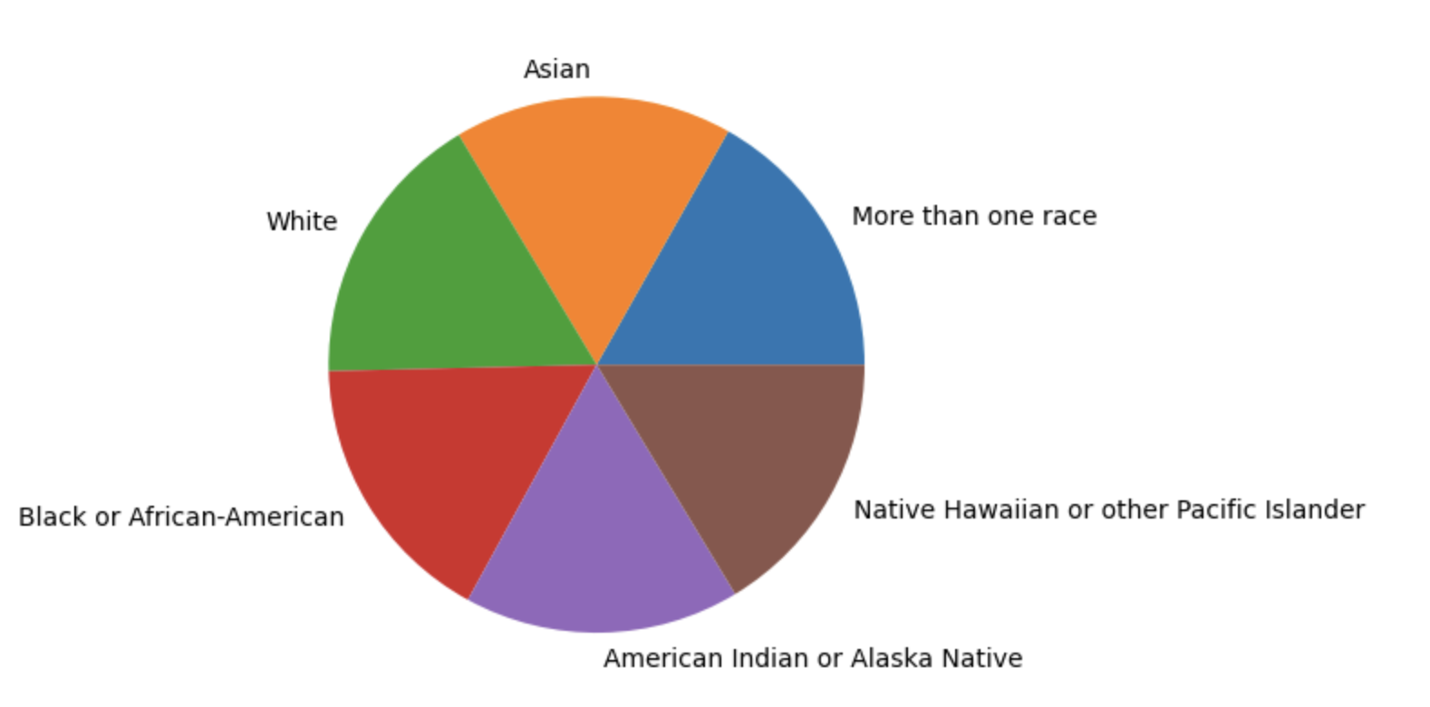
The weirdness of the age distribution
- There are only two features with continuous data: donor age and patient age.
- The patient age histogram shows that the patient age distribution has five modes(최빈값).
- Such a distribution is highly unnatural — it must be an artefact of the synthetic data generation.
plt.figure(figsize=(12, 3))
plt.subplot(1, 2, 1)
plt.hist(train.donor_age, bins=50, color='skyblue')
plt.title('Donor age histogram')
plt.xlabel('donor_age')
plt.ylabel('count')
plt.subplot(1, 2, 2)
plt.title('Patient age histogram')
plt.hist(train.age_at_hct, bins=50, color='skyblue')
plt.xlabel('age_at_hct')
plt.tight_layout()
plt.savefig('a.png')
plt.show()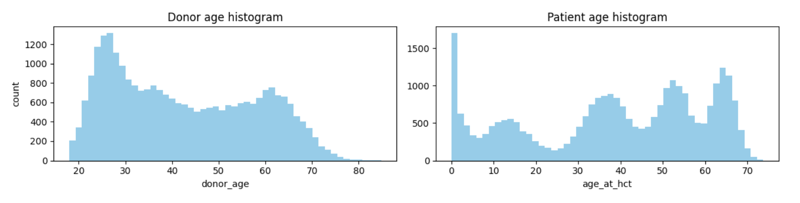
- My first thought was that different race groups had different modes, but the patient age distribution has the same five modes in every race group:
_, axs = plt.subplots(3, 2, sharex=True, sharey=True, figsize=(12, 9))
for race_group, ax in zip(race_groups, axs.ravel()):
    ax.hist(train.age_at_hct[train.race_group == race_group],
            bins=np.linspace(0, 74, 38),
            color='skyblue', alpha=0.5)
    ax.set_title(f'Patient age histogram for {race_group}')
    ax.set_xlabel('age_at_hct')
    ax.set_ylabel('count')
plt.tight_layout()
plt.savefig('b.png')
plt.show()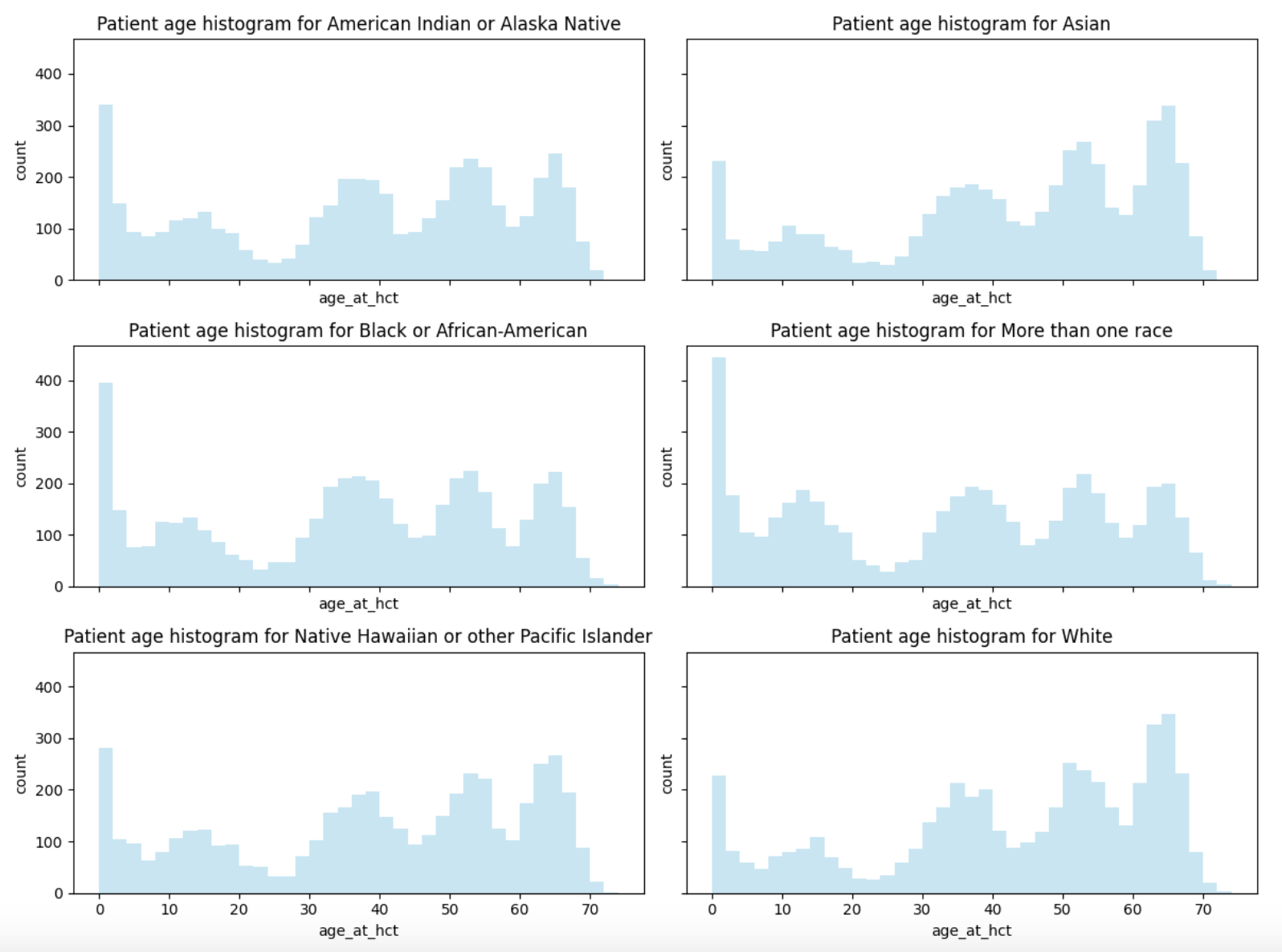
- Even stranger: The age of 0.044 years (i.e., 16 days) occurs 1005 times in the training dataset, whereas every other age occurs at most six times.
- Is hematopoietic cell transplantation a treatment which is often done to newborns? Possible.
- But I can't believe that these babies are all treated exactly when they are 16 days old.
train.age_at_hct.value_counts().sort_values(ascending=False).head()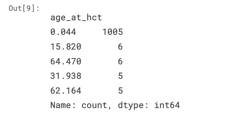
The target
The prediction target consists of two parts:
- efs_time, always positive, is a time, measured in months.
- efs, always zero or one, indicates the presence or absence of an event:
- efs=1 means "patient died exactly at time efs_time.
- actually not "died" but event occurred is the right expression
- efs=0 means "patient still lives at time efs_time; in other words, "patient dies at an unknown time strictly greater than efs_time"
- efs=1 means "patient died exactly at time efs_time.
- This situation is called "censored data": Samples of which we know the time of death are uncensored, and if we only know a lower bound for the time of death, the sample is (right-)censored.
- Censoring is the main reason that this competition has a special metric and that we need special models.
- The competition is a regression task, but we know y_true for only half the samples.
- For the other (censored) half, all we know is lower bounds for y_true.
- One cannot compute a squared error based on y_true > 100 and y_pred == 120.
- RMSE and similar metrics cannot deal with that.
- By the way, the column name is misleading: If a column is called "event-free survival", I'd expect that 0 means "patient died" and 1 means "patient lives", but that's wrong.
- The data have been obfuscated(애매함).
- efs_time is a float with three digits after the decimal point, and I don't think that events such as the death of a patient are recorded with such an exact timestamp.
- A histogram of the target values shows that half the patients die within 20 months after the transplantation; but the other half, who survives the first 20 months, has a high probability of living much longer.
plt.figure(figsize=(6, 3))
plt.hist(train.efs_time[train.efs == 0], bins=np.linspace(0, 160, 41), label='efs=0: patient still lives at this time', alpha=0.5)
plt.hist(train.efs_time[train.efs == 1], bins=np.linspace(0, 160, 41), label='efs=1: patient dies at this time', alpha=0.5)
plt.legend()
plt.xlabel('efs_time')
plt.ylabel('count')
plt.title('Target histogram')
plt.show()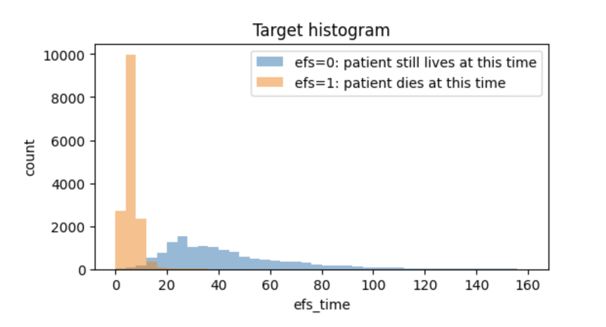
Survival function and cumulative hazard function
- The survival function shows how many patients survive for how long (Wikipedia: Kaplan–Meier estimator).
- At month 0, 100 % of the patients live.
- At month 20, only 40 % – 60 % remain, depending on their race group.
- Patients with "more than one race" have the highest probability of survival, whites the lowest.
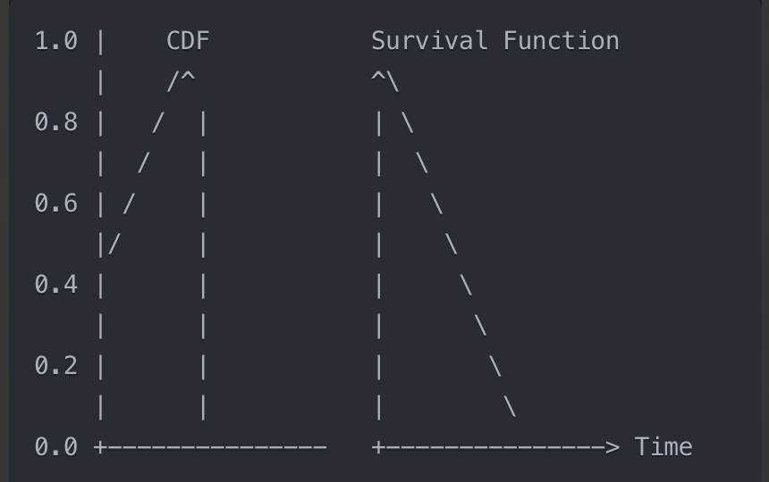
- For those who are used to working with cumulative density functions (cdf) of probability distributions, the survival function is nothing else than a top–down mirrored cdf of the time-of-event probability distribution.
- # CDF (Cumulative Distribution Function)
- Probability that an event occurs by time t
- Starts at 0 and increases upward (0 → 1)
# Survival Function
- Probability of surviving beyond time t
- Starts at 1 and decreases downward (1 → 0)
# Relationship
S(t) = 1 - F(t) where F(t) is CDF
- # CDF (Cumulative Distribution Function)
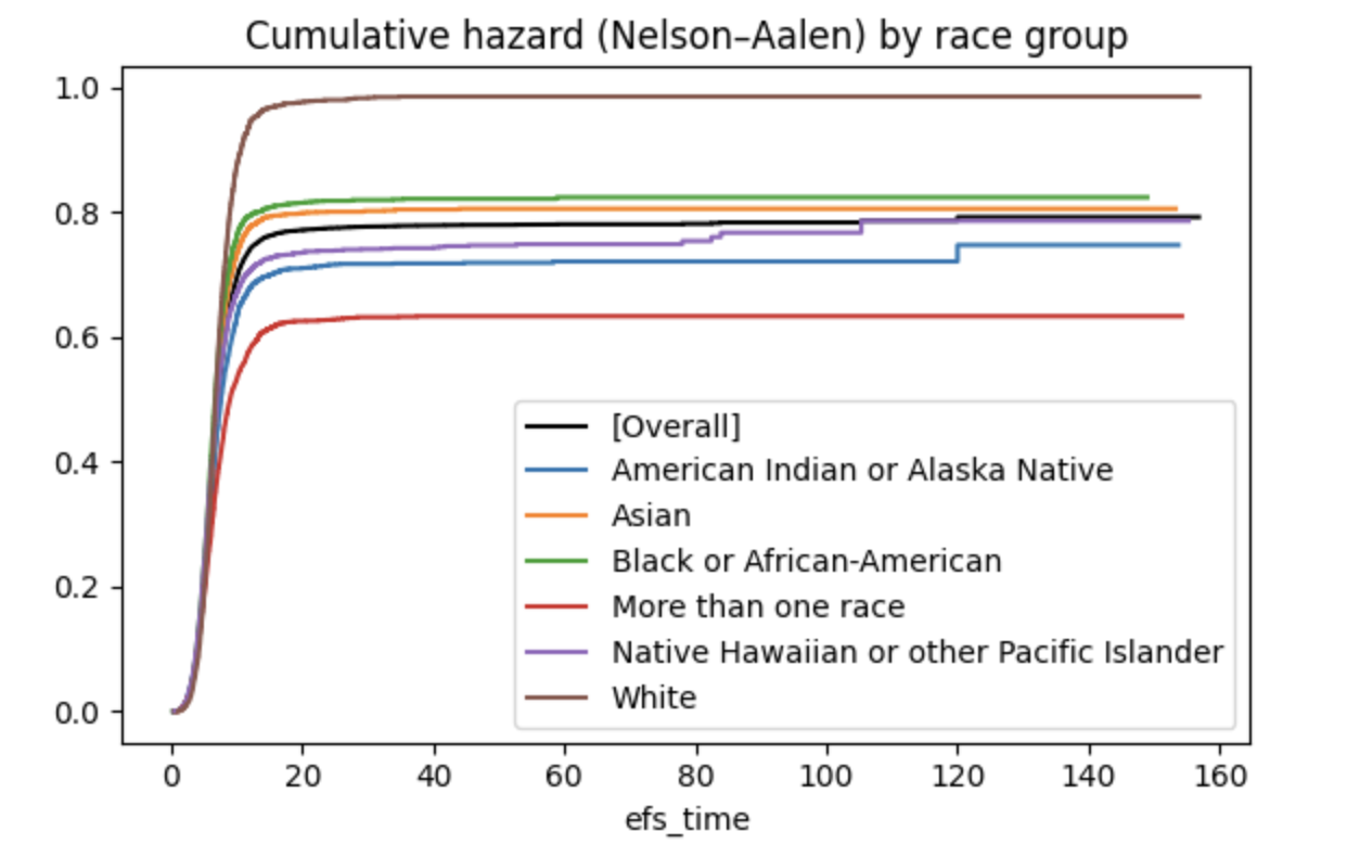
- The cumulative hazard is another representation of the same facts; it corresponds to the negative logarithm of the survival function (Wikipedia: Nelson–Aalen estimator).
- H(t) = -log(S(t))
where:
- H(t): Cumulative hazard function
- S(t): Survival function
- log: Natural logarithm
Characteristics:
- H(t) starts at 0 and increases
- As S(t) decreases, H(t) increases more rapidly - # Values over time
Time(t) | S(t) | H(t) = -log(S(t))
0 | 1.0 | 0
10 | 0.8 | 0.223
20 | 0.6 | 0.511
30 | 0.4 | 0.916
40 | 0.2 | 1.609 - These two functions express the same information in different ways:
- Survival function: Directly shows survival probability
- Cumulative hazard: Shows accumulated risk on a log scale
- Survival function: Directly shows survival probability
- These different representations are useful for emphasizing or analyzing different aspects of the data.
- H(t) = -log(S(t))
# You can use library functions or write the few lines of code yourself
# !pip install -q scikit-survival
# from sksurv.nonparametric import kaplan_meier_estimator, nelson_aalen_estimator
# from lifelines import KaplanMeierFitter

def survival_function(df):
    survival_df = df[['efs', 'efs_time']].groupby('efs_time').agg(['size', 'sum']).droplevel(0, axis=1).astype(int)
    survival_df['n_at_risk'] = survival_df['size'].sum() - survival_df['size'].shift().fillna(0).cumsum().astype(int)
    hazard = survival_df['sum'] / survival_df['n_at_risk']
    survival_df['cumulative_hazard'] = np.cumsum(hazard) # nelson_aalen_estimator
    survival_df['survival_probability'] = (1 - hazard).cumprod() # kaplan_meier_estimator
    return survival_df

plt.figure(figsize=(6, 8))

plt.subplot(2, 1, 1)
survival_df = survival_function(train)
plt.step(survival_df.index, survival_df['survival_probability'], c='k', where="post", label='[Overall]')
plt.xlabel('efs_time')
for race_group in race_groups:
    subset = train.query('race_group == @race_group')
    survival_df = survival_function(subset)
    plt.step(survival_df.index, survival_df['survival_probability'], where="post", label=race_group)
plt.xlabel('efs_time')
plt.legend(loc='upper right')
plt.title('Survival function (Kaplan–Meier) by race group')
plt.gca().yaxis.set_major_formatter(PercentFormatter(xmax=1, decimals=0)) # percent of xmax

plt.subplot(2, 1, 2)
survival_df = survival_function(train)
plt.step(survival_df.index, survival_df['cumulative_hazard'], c='k', where="post", label='[Overall]')
plt.xlabel('efs_time')
for race_group in race_groups:
    subset = train.query('race_group == @race_group')
    survival_df = survival_function(subset)
    plt.step(survival_df.index, survival_df['cumulative_hazard'], where="post", label=race_group)
plt.xlabel('efs_time')
plt.legend(loc='lower right')
plt.title('Cumulative hazard (Nelson–Aalen) by race group')

plt.tight_layout()
plt.show()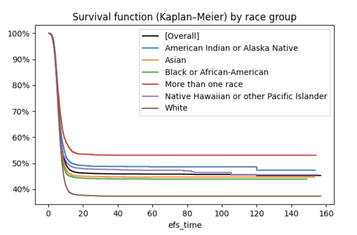
Cross-validation
- This competition is about equity in the predictions.
- This means that we score the predictions per race group and then derive the final score from these six sub-scores.
- As the official implementation of the competition metric doesn't output the scores per race group, I've written my own implementation, which gives more transparency.
- There are two main methods for survival analysis (the proportional hazards model and the accelerated failure time model), and both are implemented in XGBoost and in CatBoost.
- The calling conventions are a bit unusual.
- We present the cross-validation of six models:
- Proportional hazards model (Cox regression) with XGBoost
- This model expects that the two target columns be combined into one (y = np.where(train.efs == 1, train.efs_time, -train.efs_time), negative target values are considered right censored)
- Proportional hazards model with CatBoost.
- This model expects the targets in the same format as the XGBoost Cox model.
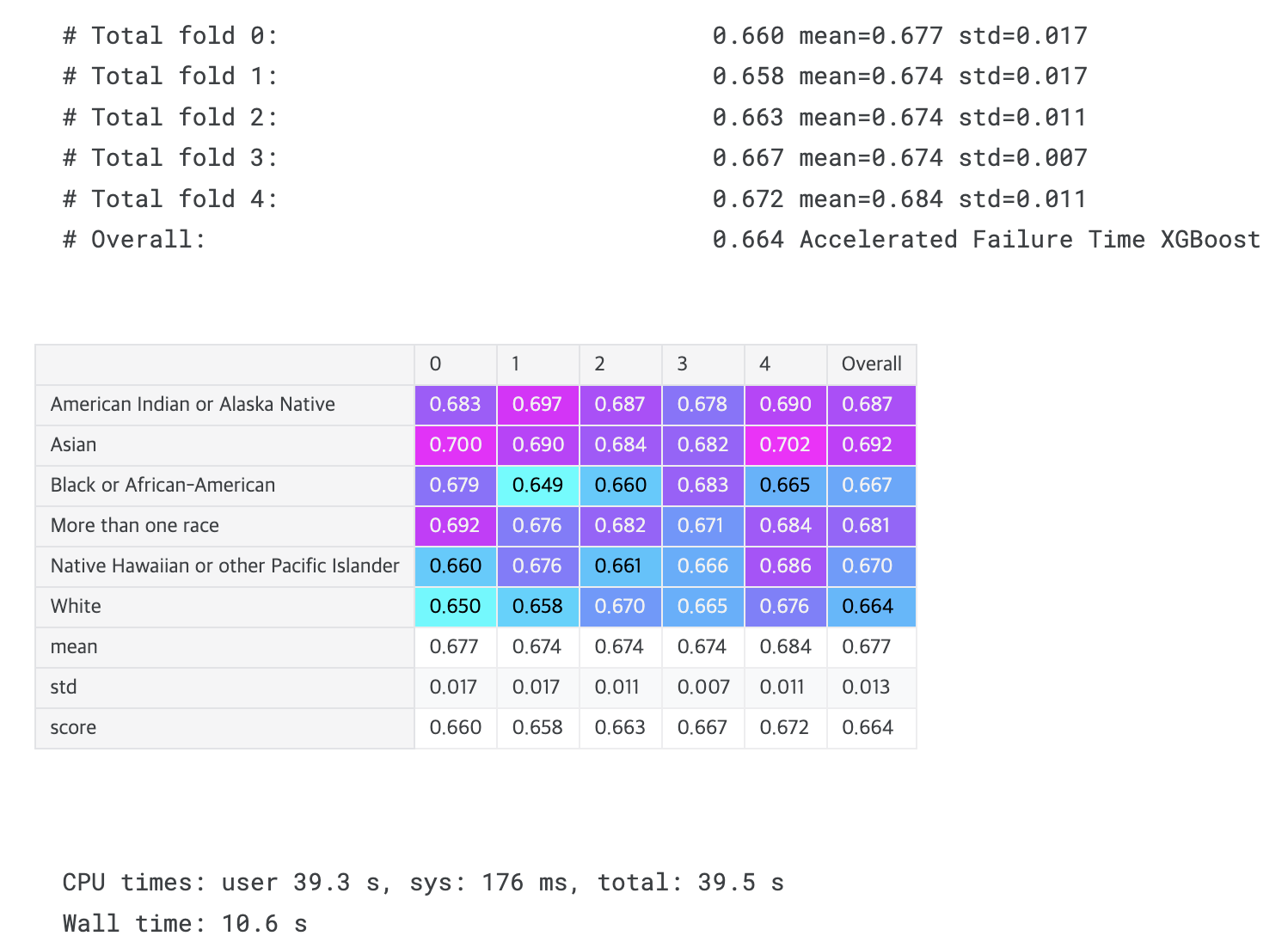
- Accelerated failure time model with XGBoost.
- This model expects the lower and upper bounds for the target in a special form in a DMatrix.
- Accelerated failure time model with CatBoost.
- This model expects the lower and upper bounds for the target in the form of a two-column array.
- Proportional hazards model with a linear implementation.
- This model expects time and event columns in a dataframe.
- MSE regression model with three different target transformations.
You'll find a comparison of the cv scores of these models at the end of the notebook.
Some hyperparameters have been taken from other public notebooks.
# from metric import score # This is the official metric which we don't use here

kf = StratifiedKFold(shuffle=True, random_state=1)

def evaluate_fold(y_va_pred, fold):
    """Compute and print the metrics (concordance index) per race group for a single fold.

    Global variables:
    - train, X_va, idx_va
    - The metrics are saved in the global list all_scores.
    """
    metric_list = []
    for race in race_groups:
        mask = X_va.race_group.values == race
        c_index_race = concordance_index(
            train.efs_time.iloc[idx_va][mask],
            - y_va_pred[mask],
            train.efs.iloc[idx_va][mask]
        )
        # print(f"# {race:42} {c_index_race:.3f}")
        metric_list.append(c_index_race)
    fold_score = np.mean(metric_list) - np.sqrt(np.var(metric_list))
    print(f"# Total fold {fold}:{' ':29} {fold_score:.3f} mean={np.mean(metric_list):.3f} std={np.std(metric_list):.3f}")
    all_scores.append(metric_list)

def display_overall(label):
    """Compute and print the overall metrics (concordance index)"""
    df = pd.DataFrame(all_scores, columns=race_groups)
    df['mean'] = df[race_groups].mean(axis=1)
    df['std'] = np.std(df[race_groups], axis=1)
    df['score'] = df['mean'] - df['std']
    df = df.T
    df['Overall'] = df.mean(axis=1)
    temp = df.drop(index=['std']).values
    print(f"# Overall:                                   {df.loc['score', 'Overall']:.3f} {label}")
    all_model_scores[label] = df.loc['score', 'Overall']
    display(df
            .iloc[:len(race_groups)]
            .style
            .format(precision=3)
            .background_gradient(axis=None, vmin=temp.min(), vmax=temp.max(), cmap="cool")
            .concat(df.iloc[len(race_groups):].style.format(precision=3))
           )
%%time
# XGBoost Cox regression
y = np.where(train.efs == 1, train.efs_time, -train.efs_time)
all_scores = []
for fold, (idx_tr, idx_va) in enumerate(kf.split(train, train.race_group)):
X_tr = train.iloc[idx_tr][features]
X_va = train.iloc[idx_va][features]
y_tr = y[idx_tr]
xgb_cox_params = {'objective': 'survival:cox', 'grow_policy': 'depthwise',
'n_estimators': 700, 'learning_rate': 0.0254, 'max_depth': 8,
'reg_lambda': 0.116, 'reg_alpha': 0.139, 'min_child_weight': 23.8,
'colsample_bytree': 0.59, 'subsample': 0.7, 'tree_method': 'hist',
'enable_categorical': True}
model = xgboost.XGBRegressor(**xgb_cox_params)
model.fit(X_tr, y_tr) # negative values are considered right censored
y_va_pred = model.predict(X_va) # predicts hazard factor
evaluate_fold(y_va_pred, fold)
display_overall('Cox Proportional Hazards XGBoost')
# Overall: 0.670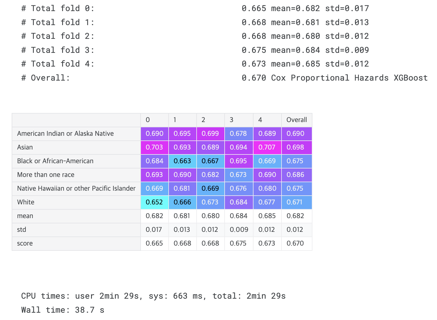
%%time
# Catboost Cox regression
y = np.where(train.efs == 1, train.efs_time, -train.efs_time)
all_scores = []
for fold, (idx_tr, idx_va) in enumerate(kf.split(train, train.race_group)):
    X_tr = train.iloc[idx_tr][features]
    X_va = train.iloc[idx_va][features]
    y_tr = y[idx_tr]

    cb_cox_params = {'loss_function': 'Cox', 'grow_policy': 'SymmetricTree',
                     'n_estimators': 800, 'learning_rate': 0.092, 'l2_leaf_reg': 2.5,
                     'max_depth': 7, 'colsample_bylevel': 0.84, 'subsample': 0.9,
                     'random_strength': 0.8, 'verbose': False}

    model = catboost.CatBoostRegressor(**cb_cox_params, cat_features=cat_features)
    model.fit(X_tr, y_tr)
    y_va_pred = model.predict(X_va) # predicts log of hazard factor
    evaluate_fold(y_va_pred, fold)
display_overall('Cox Proportional Hazards CatBoost')
# Overall:                                   0.669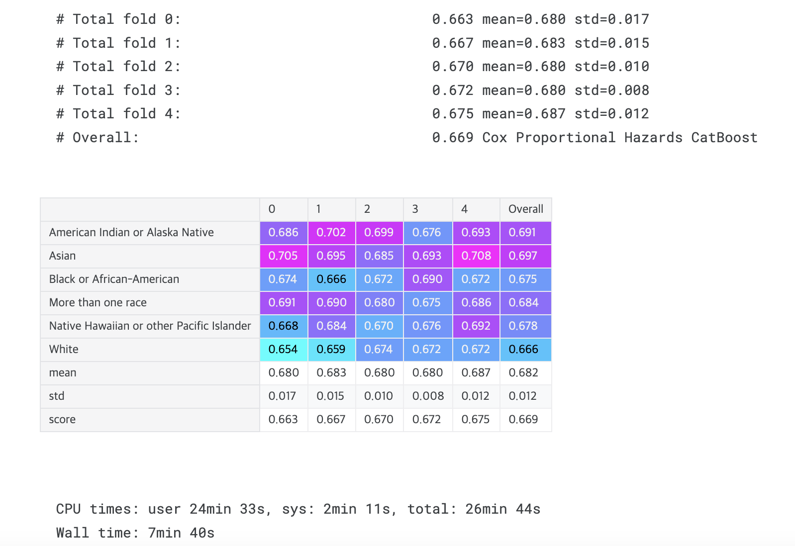
%%time
# XGBoost Accelerated failure time model
all_scores = []

# Data split and preparation
for fold, (idx_tr, idx_va) in enumerate(kf.split(train, train.race_group)):
    # K-fold cross-validation stratified by race_group
    X_tr = train.iloc[idx_tr][features]
    X_va = train.iloc[idx_va][features]

    # Creating xgboost data matrix
    d_tr = xgboost.DMatrix(X_tr, enable_categorical=True)
    # Setting survival time information for AFT model
    d_tr.set_float_info('label_lower_bound', train.efs_time.iloc[idx_tr])
    d_tr.set_float_info('label_upper_bound', np.where(train.efs.iloc[idx_tr] == 0, np.inf, train.efs_time.iloc[idx_tr]))

    d_va = xgboost.DMatrix(X_va, enable_categorical=True)
    d_va.set_float_info('label_lower_bound', train.efs_time.iloc[idx_va])
    d_va.set_float_info('label_upper_bound', np.where(train.efs.iloc[idx_va] == 0, np.inf, train.efs_time.iloc[idx_va]))

    # Model parameters setting
    xgboost_aft_params = {'learning_rate': 0.08, 'max_depth': 4, 'reg_lambda': 3, 'aft_loss_distribution_scale': 0.9,
                          'reg_alpha': 0.24, 'gamma': 0.033, 'min_child_weight': 82.58861553592878,
                          'colsample_bytree': 0.5662198438953138, 'max_bin': 53, 'subsample': 0.7456329821182728,
                          'objective': 'survival:aft', 'grow_policy': 'depthwise', 'tree_method': 'hist',
                          'aft_loss_distribution': 'normal'}
    # Model training
    bst = xgboost.train(xgboost_aft_params,
                        d_tr,
                        num_boost_round=300,
                        # evals=[(d_tr, 'train'), (d_va, 'val')],
                       )

    # Prediction & Evaluation
    y_va_pred = - bst.predict(d_va) # model predicts time of death
    # Taking negative because: converting to risk score
    # Earlier death time means higher risk
    evaluate_fold(y_va_pred, fold)
display_overall('Accelerated Failure Time XGBoost')
# Overall: 0.664- d_tr = xgboost.DMatrix(X_tr, enable_categorical=True)
- Creates DMatrix, XGBoost's specialized data format
- enable_categorical=True: Automatically handles categorical variables
- d_tr.set_float_info('label_lower_bound', train.efs_time.iloc[idx_tr])
- Setting survival time lower bound = label_lower_bound
- Sets observed time (efs_time) as lower bound for all patients
- Means the patient survived at least until this time, regardless of whether event occurred (efs=1) or was censored (efs=0)
- d_tr.set_float_info('label_upper_bound', np.where(train.efs.iloc[idx_tr] == 0, np.inf, train.efs_time.iloc[idx_tr]))
- Setting survival time upper bound = label_upper_bound
- Splits into 2 cases:
- efs=1 (event occurred):
- upper_bound = efs_time
# We know the exact time of death
- upper_bound = efs_time
- efs=0 (censored):
- upper_bound = np.inf (infinity)
# We don't know when death occurred after last observation
- upper_bound = np.inf (infinity)
- efs=1 (event occurred):
- Actually setting the upper and lower bound of survival time for validation data is unnecessary
- Example:
- # Patient A: died on day 100 (efs=1)
lower_bound = 100
upper_bound = 100
# Means death occurred exactly at 100 days
# Patient B: censored on day 80 (efs=0)
lower_bound = 80
upper_bound = inf
# Means survived at least 80 days, unknown after that
- # Patient A: died on day 100 (efs=1)
%%time
# CatBoost Accelerated failure time model
y = np.column_stack([train.efs_time,
                     np.where(train.efs == 1, train.efs_time, -1)])
all_scores = []
for fold, (idx_tr, idx_va) in enumerate(kf.split(train, train.race_group)):
    X_tr = train.iloc[idx_tr][features]
    X_va = train.iloc[idx_va][features]
    y_tr = y[idx_tr]
    cb_aft_params = {'loss_function': 'SurvivalAft', 'grow_policy': 'SymmetricTree',
                     'n_estimators': 800, 'learning_rate': 0.066, 'l2_leaf_reg': 4.4,
                     'max_depth': 5, 'colsample_bylevel': 0.776, 'random_strength': 0.9,
                     'verbose': False} # 0.67551
    model = catboost.CatBoostRegressor(**cb_aft_params, cat_features=cat_features)
    model.fit(X_tr, y_tr)
    y_va_pred = - model.predict(X_va) # model predicts log of time of death
    evaluate_fold(y_va_pred, fold)
display_overall('Accelerated Failure Time CatBoost')
# Overall:                                   0.664
Target transformation models and regression with mean squared error
- The competition task can be interpreted as predicting the order of death of the patients.
- Who dies first? Who dies second? ... Who dies last, and who survives?
- With a suitable target transformation, we can apply the usual regression algorithms which optimize mse or similar metrics.
- In the public notebooks of this competition, we can find various target transformations, but they all are similar.
- Patients who die mostly have an efs_time between 0 and 15, whereas most survivors have an efs_time between 15 and 160.
- This distribution is an impediment for regression models.
- We want predictions to have high discriminative power for the patients who die, but we don't need to distinguish between survivors.
- We can achieve this result by stretching the range of the patients who die and compressing the range of the survivors.
- The diagram shows how a typical target transformation stretches and compresses the ranges:
def transform_survival_probability(time, event):
    """Transform the target by stretching the range of eventful efs_times and compressing the range of event_free efs_times

    From https://www.kaggle.com/code/cdeotte/gpu-lightgbm-baseline-cv-681-lb-685
    """
    kmf = KaplanMeierFitter()
    kmf.fit(time, event)
    y = kmf.survival_function_at_times(time).values
    return y

y_quantile = transform_survival_probability(time=train.efs_time, event=train.efs)
survival_df = survival_function(train)

fig, axs = plt.subplots(2, 2, figsize=(10, 10), dpi=80)

axs[0, 0].hist(train.efs_time[train.efs == 0], bins=np.linspace(0, 160, 41), label='efs=0: patient still lives at this time', alpha=0.5)
axs[0, 0].hist(train.efs_time[train.efs == 1], bins=np.linspace(0, 160, 41), label='efs=1: patient dies at this time', alpha=0.5)
axs[0, 0].legend()
axs[0, 0].set_xlabel('efs_time')
axs[0, 0].set_ylabel('count')
axs[0, 0].set_title('Original target histogram')

axs[0, 1].set_axis_off()

axs[1, 0].step(survival_df.index, survival_df['survival_probability'], c='k', lw=3, where="post", label='[Overall]')
axs[1, 0].set_xlabel('efs_time')
axs[1, 0].set_ylabel("quantile")
axs[1, 0].set_title("Survival function")
axs[1, 0].yaxis.set_major_formatter(PercentFormatter(xmax=1, decimals=0))

axs[1, 1].hist(y_quantile[train.efs==0], bins=100, label="efs=0", orientation=u'horizontal', alpha=0.5)
axs[1, 1].hist(y_quantile[train.efs==1], bins=100, label="efs=1", orientation=u'horizontal', alpha=0.5)
axs[1, 1].legend()
axs[1, 1].set_ylabel("quantile")
axs[1, 1].set_xlabel("count")
axs[1, 1].set_title("Transformed target histogram (sideways)")
axs[1, 1].yaxis.set_major_formatter(PercentFormatter(xmax=1, decimals=0))

ax = plt.Axes(fig, [0., 0., 1., 1.])
ax.set_axis_off()
ax.set_xlim(0, 1)
ax.set_ylim(0, 1)
fig.add_axes(ax)
ax.arrow(0.2, 0.55, 0, -0.47, length_includes_head=True, width=0.002, color=plt.get_cmap('tab10')(0), alpha=0.5, head_width=0.02, head_length=0.02)
ax.arrow(0.2, 0.082, 0.37, 0, length_includes_head=True, width=0.002, color=plt.get_cmap('tab10')(0), alpha=0.5, head_width=0.02, head_length=0.02)
ax.arrow(0.12, 0.55, 0, -0.3, length_includes_head=True, width=0.002, color=plt.get_cmap('tab10')(1), alpha=0.5, head_width=0.02, head_length=0.02)
ax.arrow(0.12, 0.25, 0.45, 0, length_includes_head=True, width=0.002, color=plt.get_cmap('tab10')(1), alpha=0.5, head_width=0.02, head_length=0.02)

plt.suptitle('Transforming the target', y=0.99, size=20)
with warnings.catch_warnings():
    warnings.simplefilter("ignore")
    plt.tight_layout()
plt.show()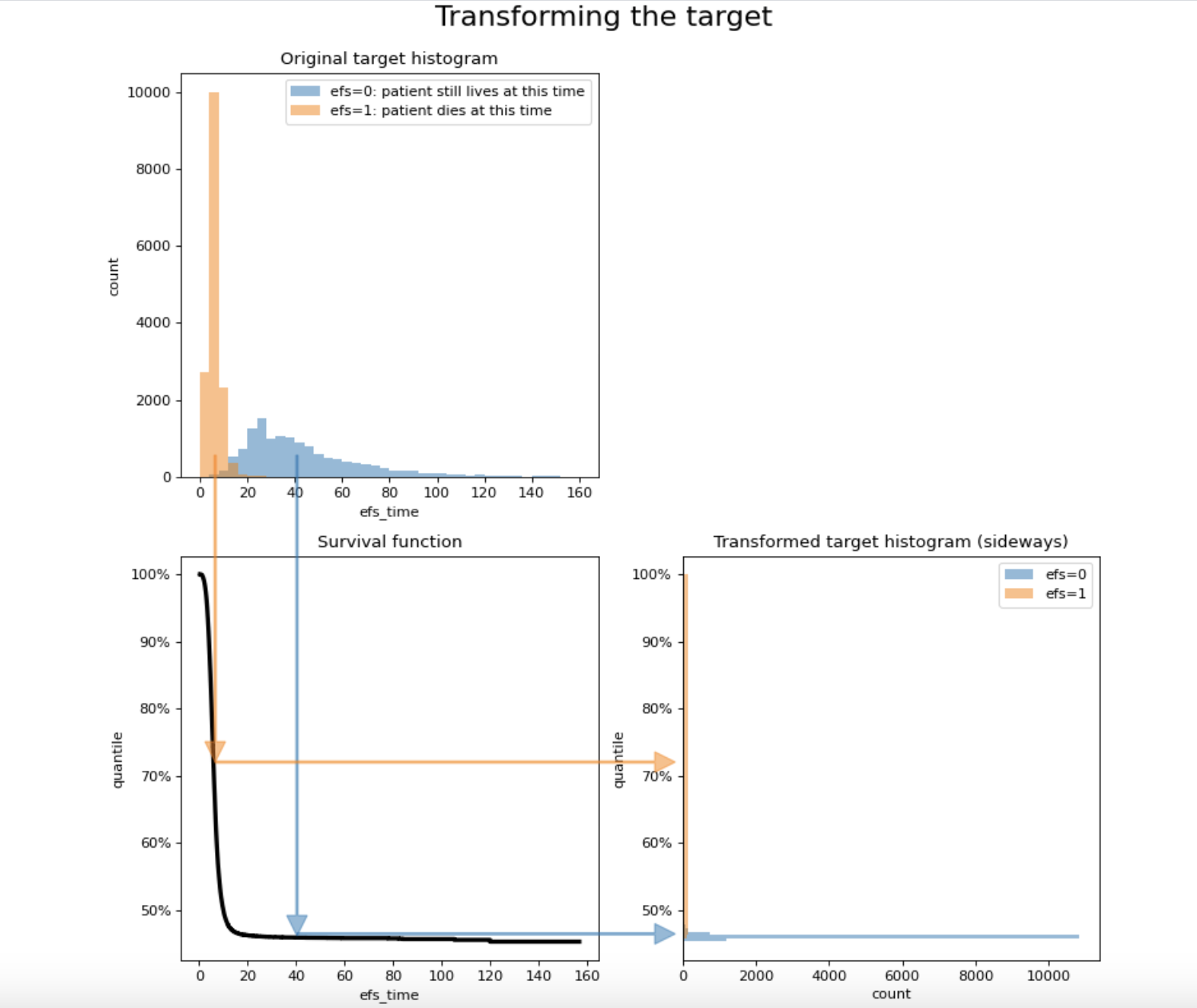
- What we already saw from my discussion annotation: https://dongsunseng.com/entry/CIBMTR-Equity-in-post-HCT-Survival-Predictions-8-Finding-the-best-target-transformation
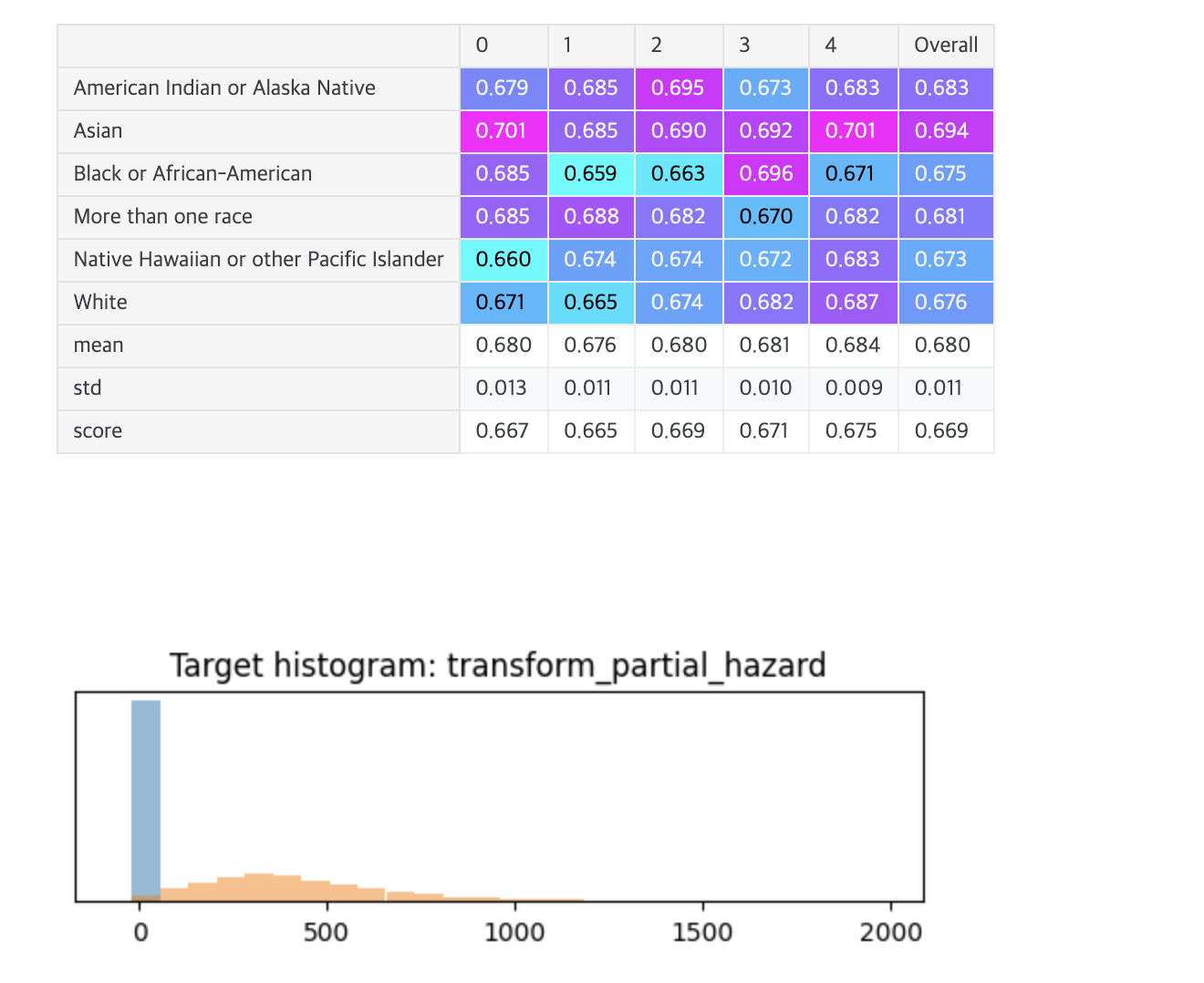
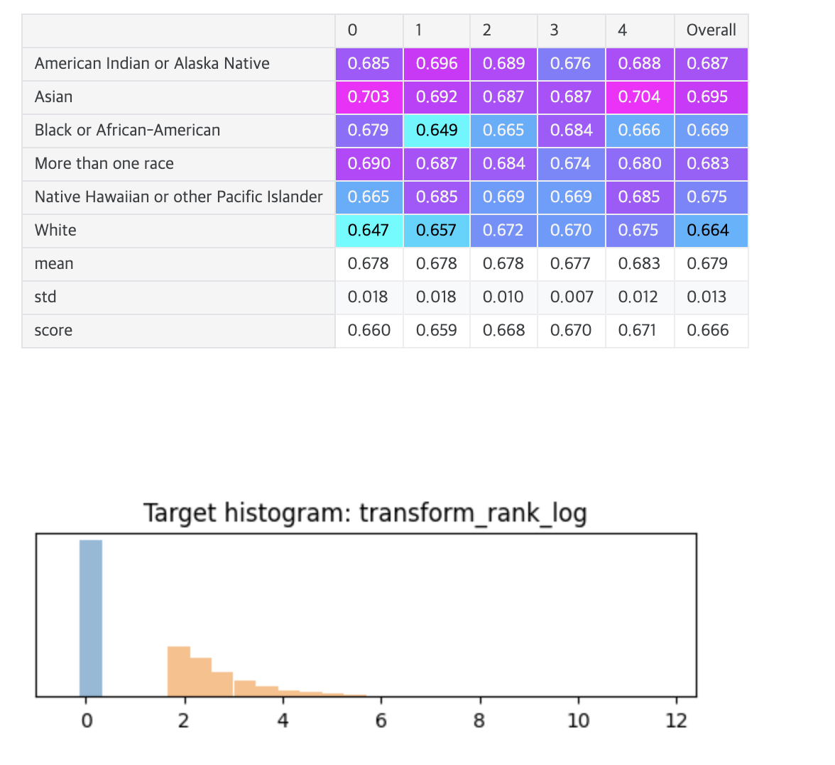
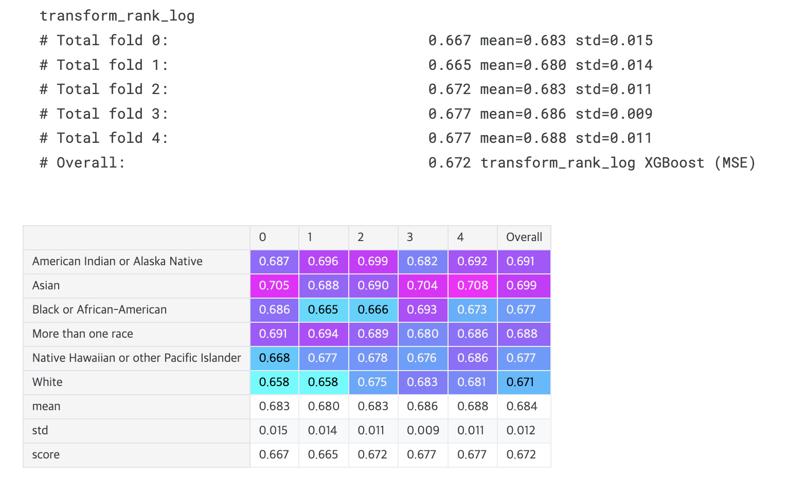
- We now plot the histograms of five possible transformations and then fit regression models with MSE loss to each of the transformed targets.
- You can of course try other loss functions and see what happens.
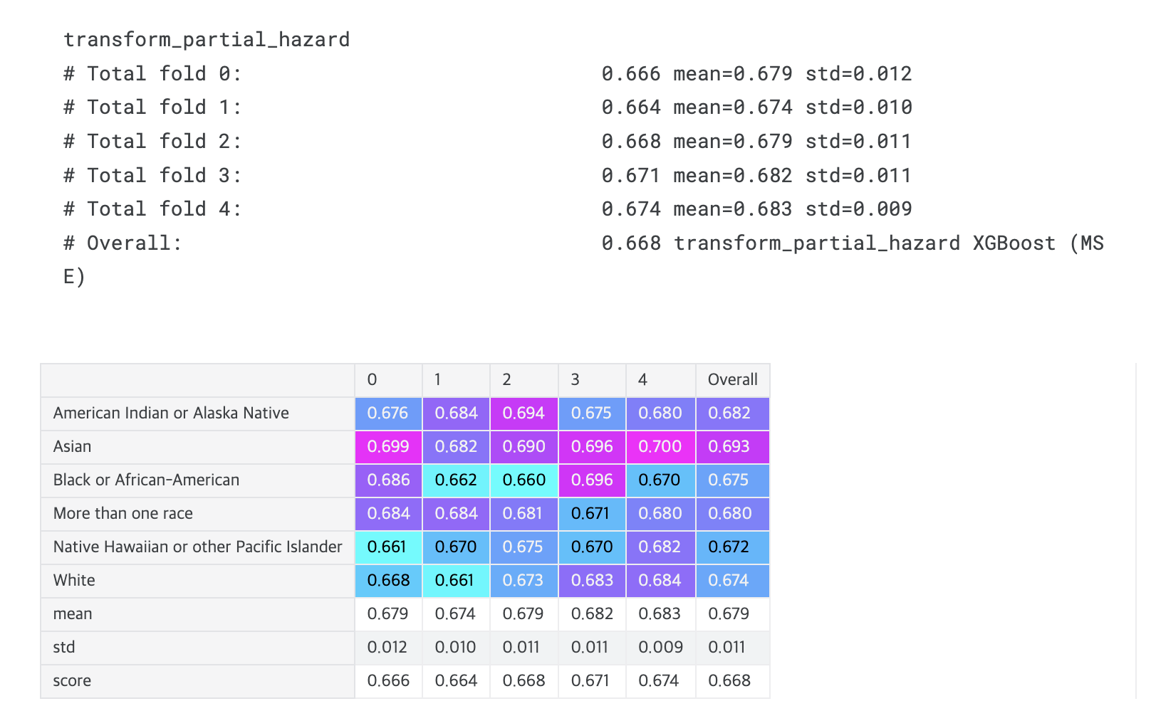
def transform_partial_hazard(time, event):
"""Transform the target by stretching the range of eventful efs_times and compressing the range of event_free efs_times
From https://www.kaggle.com/code/andreasbis/cibmtr-eda-ensemble-model
"""
data = pd.DataFrame({'efs_time': time, 'efs': event, 'time': time, 'event': event})
cph = CoxPHFitter()
with warnings.catch_warnings():
warnings.simplefilter("ignore")
cph.fit(data, duration_col='time', event_col='event')
return cph.predict_partial_hazard(data)
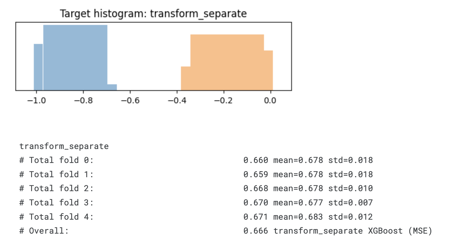
def transform_separate(time, event):
"""Transform the target by separating events from non-events
From https://www.kaggle.com/code/mtinti/cibmtr-lofo-feature-importance-gpu-accelerated"""
transformed = time.values.copy()
mx = transformed[event == 1].max() # last patient who dies
mn = transformed[event == 0].min() # first patient who survives
transformed[event == 0] = time[event == 0] + mx - mn
transformed = rankdata(transformed)
transformed[event == 0] += len(transformed) // 2
transformed = transformed / transformed.max()
return - transformed
def transform_rank_log(time, event):
"""Transform the target by stretching the range of eventful efs_times and compressing the range of event_free efs_times
From https://www.kaggle.com/code/cdeotte/nn-mlp-baseline-cv-670-lb-676"""
transformed = time.values.copy()
mx = transformed[event == 1].max() # last patient who dies
mn = transformed[event == 0].min() # first patient who survives
transformed[event == 0] = time[event == 0] + mx - mn
transformed = rankdata(transformed)
transformed[event == 0] += len(transformed) * 2
transformed = transformed / transformed.max()
transformed = np.log(transformed)
return - transformed
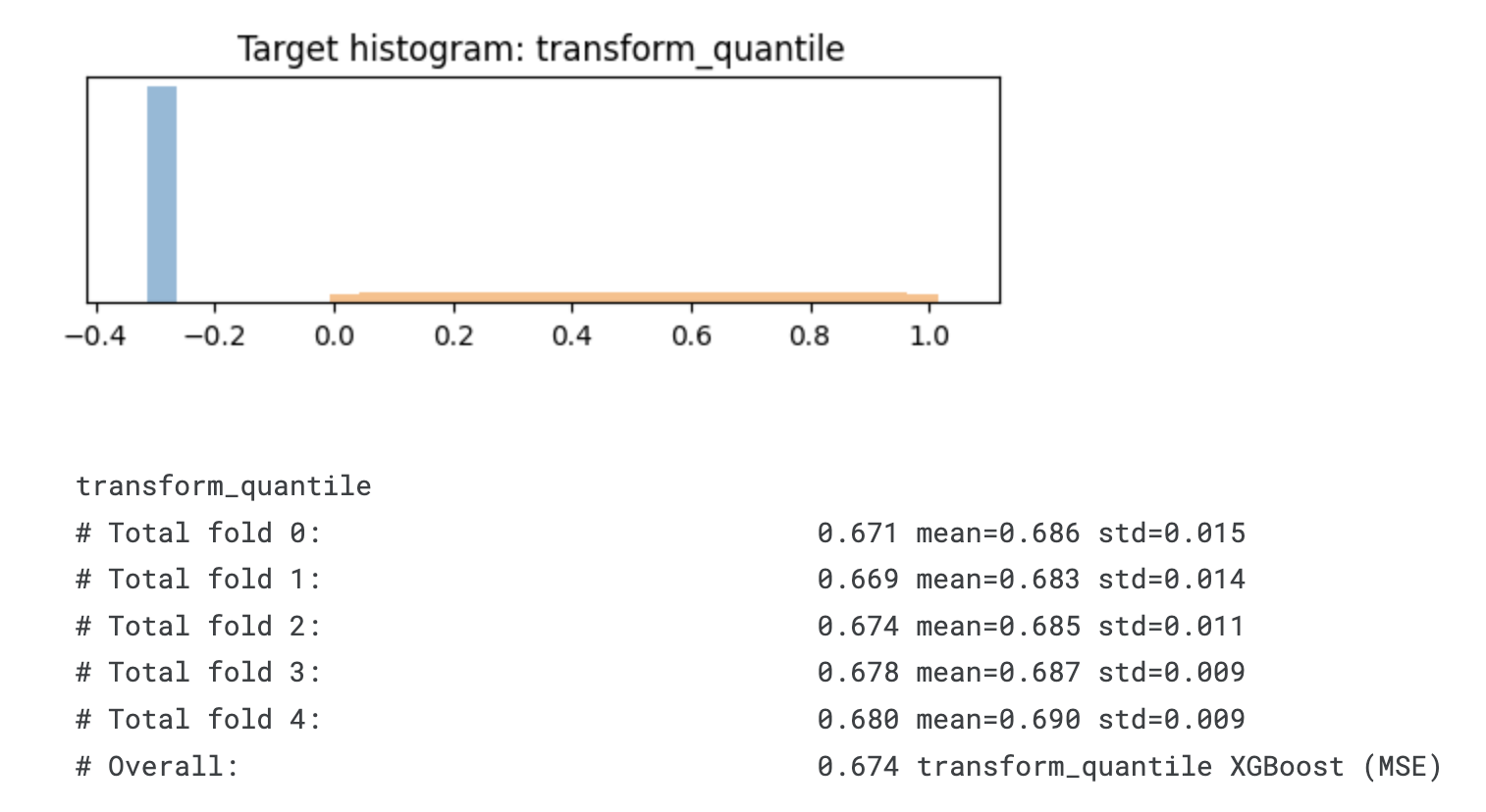
def transform_quantile(time, event):
"""Transform the target by stretching the range of eventful efs_times and compressing the range of event_free efs_times
From https://www.kaggle.com/code/ambrosm/esp-eda-which-makes-sense"""
transformed = np.full(len(time), np.nan)
transformed_dead = quantile_transform(- time[event == 1].values.reshape(-1, 1)).ravel()
transformed[event == 1] = transformed_dead
transformed[event == 0] = transformed_dead.min() - 0.3
return transformed# XGBoost: MSE loss with five different target transformations
for transformation in [transform_survival_probability,
transform_partial_hazard,
transform_separate,
transform_rank_log,
transform_quantile,
]:
plt.figure(figsize=(6, 1.5))
target = transformation(time=train.efs_time, event=train.efs)
vmin, vmax = 1.09 * target.min() - 0.09 * target.max(), 1.09 * target.max() - 0.09 * target.min()
plt.hist(target[train.efs == 0], bins=np.linspace(vmin, vmax, 31), density=True, label='efs=0: patient still lives at this time', alpha=0.5)
plt.hist(target[train.efs == 1], bins=np.linspace(vmin, vmax, 31), density=True, label='efs=1: patient dies at this time', alpha=0.5)
plt.xlim(vmin, vmax)
plt.yticks([])
plt.title('Target histogram: ' + transformation.__name__)
plt.show()
print(transformation.__name__)
all_scores = []
for fold, (idx_tr, idx_va) in enumerate(kf.split(train, train.race_group)):
X_tr = train.iloc[idx_tr][features]
X_va = train.iloc[idx_va][features]
y_tr = transformation(time=train.iloc[idx_tr].efs_time, event=train.iloc[idx_tr].efs)
# from https://www.kaggle.com/code/cdeotte/gpu-lightgbm-baseline-cv-681-lb-685
model = xgboost.XGBRegressor(
max_depth=3,
colsample_bytree=0.5,
subsample=0.8,
n_estimators=2000,
learning_rate=0.02,
enable_categorical=True,
min_child_weight=80,
)
model.fit(X_tr, y_tr)
y_va_pred = model.predict(X_va) # predicts quantile
evaluate_fold(y_va_pred, fold)
display_overall(f'{transformation.__name__} XGBoost (MSE)')
print()
# Overall: 0.669 transform_survival_probability
# Overall: 0.668 transform_partial_hazard
# Overall: 0.666 transform_separate
# Overall: 0.672 transform_rank_log
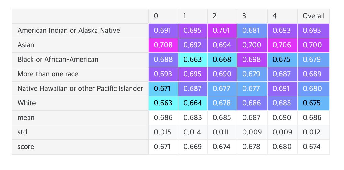
# Overall: 0.674 transform_quantile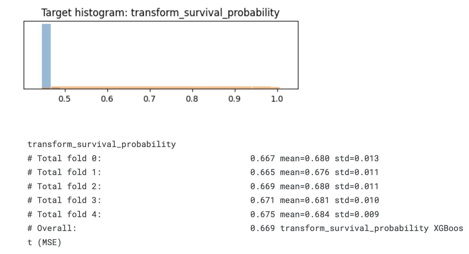
A linear model
- The linear model CoxPHFitter needs one-hot encoding and missing value imputation:
%%time
# see https://lifelines.readthedocs.io/en/latest/Survival%20Regression.html#cox-s-proportional-hazard-model

all_scores = []
for fold, (idx_tr, idx_va) in enumerate(kf.split(train, train.race_group)):
    # Creating preprocessing pipeline - one hot encoding for categorical variables
    preproc = ColumnTransformer([
    # One-hot encoding for categorical variables
    ('ohe', OneHotEncoder(
        drop='first',  # Drop first category (dummy coding)
        sparse_output=False,
        handle_unknown='ignore'),
        cat_features),
    ],
    # Replace missing values in numerical variables with median
    remainder=SimpleImputer(strategy='median')
).set_output(transform='pandas')

    # Apply data preprocessing
    X_tr = preproc.fit_transform(train.iloc[idx_tr])
    with warnings.catch_warnings():
        warnings.simplefilter("ignore")
        X_va = preproc.transform(train.iloc[idx_va])

    # Create and Train Cox model
    model = CoxPHFitter(penalizer=.01) # Apply L2 regularization
    feats = [f for f in X_tr.columns if f not in ['gvhd_proph_FK+- others(not MMF,MTX)']]
    model.fit(X_tr[feats], duration_col='efs_time', event_col='efs')
    # model.print_summary()
    y_va_pred = model.predict_partial_hazard(X_va[feats])
    X_va['race_group'] = train.race_group.iloc[idx_va]
    evaluate_fold(y_va_pred, fold)
display_overall('Cox Proportional Hazards Linear')
# Overall: 0.656- XGBoost Cox vs. CoxPHFitter
- XGBoost Cox:
- Can learn nonlinear relationships
- Can capture complex interactions between features
- Automatically handles missing values as a tree-based model
- CoxPHFitter:
- Linear model (learns only linear relationships)
- Features affect hazard independently
- Requires preprocessing (one-hot encoding, missing value handling)
- Basic Cox Model Equation:
- h(t|X) = h₀(t) * exp(β₁X₁ + β₂X₂ + ... + βₙXₙ)
# h₀(t): baseline hazard function
# βᵢ: coefficient for each feature
# Xᵢ: feature value
- h(t|X) = h₀(t) * exp(β₁X₁ + β₂X₂ + ... + βₙXₙ)
- Learns through partial likelihood func:
- Details in my previous post: https://dongsunseng.com/entry/CIBMTR-Equity-in-post-HCT-Survival-Predictions-2-Understanding-Survival-Analysis
- XGBoost Cox:
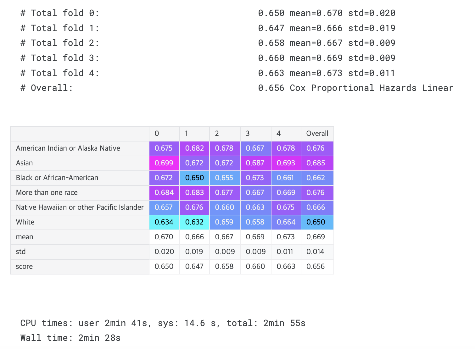
- Observation: With most models, the Asian predictions get the highest scores (best concordance index) and the predictions for white patients get the lowest scores (worst concordance).
- Insight: As the competition objective (equitability across diverse patient populations) rewards models with similar concordance scores for all six race groups, a possible strategy could be that we artificially make the predictions for Asian patients worse.
- # Stratified C-index = Mean(C-indices) - Std(C-indices)
# That is, mean of C-indices for each racial group minus their standard deviation
Example:
Race A: C-index = 0.70
Race B: C-index = 0.70
Race C: C-index = 0.70
=> Mean 0.70, Std 0 -> Final score 0.70
Race A: C-index = 0.75
Race B: C-index = 0.65
Race C: C-index = 0.70
=> Mean 0.70, Std 0.05 -> Final score 0.65 - What this insight suggests:
- If predictions for Asian patients are more accurate than other races
- Deliberately lowering the accuracy for Asian predictions
- To make performance similar across all racial groups
- Could improve the overall score
- If predictions for Asian patients are more accurate than other races
- # Stratified C-index = Mean(C-indices) - Std(C-indices)
Final comparison
- For the time being, the gradient-boosted proportional hazard models (Cox regression, blue) and the transformed-target models (pink) win.
- Among the target transformations, transform_quantile is best.
- The AFT models (green) perhaps need more hyperparameter tuning.
result_df = pd.DataFrame(all_model_scores, index=['score']).T
result_df = result_df.sort_values('score', ascending=False)
# with pd.option_context("display.precision", 3): display(result_df)
plt.figure(figsize=(6, len(result_df) * 0.4))

color = np.where(result_df.index.str.contains('Proportional'),
                 'cyan',
                 np.where(result_df.index.str.contains('Accelerated'), 'lightgreen',
                          'lightpink'))
bars = plt.barh(np.arange(len(result_df)), result_df.score, color=color)
plt.gca().bar_label(bars, fmt='%.3f')
plt.yticks(np.arange(len(result_df)), result_df.index)
plt.xlim(0.65, 0.68)
plt.xticks([0.65, 0.66, 0.67, 0.68])
plt.gca().invert_yaxis()
plt.xlabel('CV score (higher is better)')
plt.show()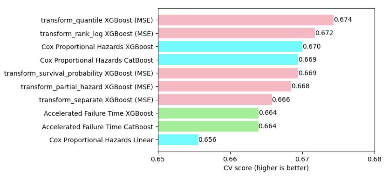
완벽해야 한다는 강박은 시작을 망친다.
반응형