CIBMTR - Equity in post-HCT Survival Predictions #9 NN Starter Notebook

Annotation of discussion and kernel for NN Solution from Chris Deotte

Discussion Link:

https://www.kaggle.com/competitions/equity-post-HCT-survival-predictions/discussion/550343

CIBMTR - Equity in post-HCT Survival Predictions

Kernel Link:

https://www.kaggle.com/code/cdeotte/nn-mlp-baseline-cv-670-lb-676

NN (MLP) Baseline - [CV 670 LB 676]

---

NN Starter Notebook CV 0.670 LB 0.676 (Discussion)

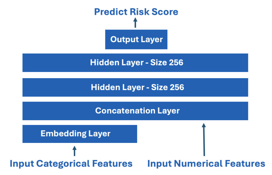
• I published a starter notebook NN which uses the following simple architecture.
• Consider improving architecture to boost CV and LB score!

Preprocessing

• There are 57 features with 35 categorical and 22 numerical.
• The majority of numerical features appear to be like categorical features with their low unique value count.
• Therefore in my NN starter, I convert 55 features into categorical leaving only donor_age and act_at_hct as numerical.
• For each categorical, we label encode.
• In the NN architecture, we use embeddings for each categorical features.
• For each categorical feature, the embedding input size is of course the number of unique values.
• The embedding output size is sqrt(number unique)+1.
  • About embedding
    • The process of converting categorical data into meaningful continuous vectors
    • Categories with similar meanings learn to have similar vector values
    • Examples:
      • # Example: Disease Type Categories
        Disease A = [0.2, 0.8, -0.3]  # Converted to 3D vector
        Disease B = [0.3, 0.7, -0.2]  # Similar diseases have similar vector values
        Disease C = [-0.8, -0.2, 0.9] # Different types have different vector values
    • Limitations of one-hot encoding:
      • # One-Hot Encoding
        Disease A = [1, 0, 0, 0]
        Disease B = [0, 1, 0, 0]
        Disease C = [0, 0, 1, 0]
        # All categories are equidistant
        # Cannot express similarity
    • Advantages of Embedding:
      • # Embedding
        Disease A = [0.2, 0.8]  # Compressed to 2D
        Disease B = [0.3, 0.7]  # Similar vector to A
        Disease C = [-0.8, -0.2]  # Different vector from A,B
        # Can express similarity through vector distances
  • The practice of setting embedding output size to sqrt(number of unique values) + 1 is a commonly used rule of thumb.
    • Example:
      • categorical_feature = 'disease_type'
        unique_values = 16  # Assuming there are 16 disease types
        embedding_output_size = int(np.sqrt(16)) + 1
        # = 4 + 1 = 5
    • Reasons for this setting:
      
      • Dimension Reduction:
        
        • One-hot encoding would require 16 dimensions
        • Embedding can reduce it to 5 dimensions
        • This reduces model complexity and makes learning more efficient
      • Appropriate Expressiveness:
        
        • Too small embedding dimension: Risk of information loss
        • Too large embedding dimension: Risk of overfitting
        • sqrt(n) + 1 is an empirical method to find balance between these
    • Real Example:
      • # Embedding dimensions for various category sizes
        4 categories -> 3 embedding dimensions  (√4 + 1)
        9 categories -> 4 embedding dimensions  (√9 + 1)
        16 categories -> 5 embedding dimensions (√16 + 1)
        25 categories -> 6 embedding dimensions (√25 + 1)
• Afterward we concatenate all the categorical embeddings together with the numerical features and continue forward with MLP.
• For the two numericals, we standardize with feature = (feature - mean)/std because NN like standardized features.

Target Transformation

• There are two ways to train a Survival Model:
  • We can input both efs and efs_time and use survival loss like Cox.
  • Transform efs and efs_time into a single target proxy for risk score and train with regression loss like MSE.
• In my NN starter, I employ option 2 above.
• I transform the original two targets into a proxy for risk score and train NN with MSE regression loss.
• Below shows the original two targets and the new transformed target.
• When training with MSE loss, the model likes the target to be like Gaussian distribution.
• This was one factor when I invented this new way to transform target:

---

NN (MLP) Baseline - [CV 670 LB 676] (Kernel)

Intro

• In this notebook, we present a Neural Network NN (MLP) baseline.
• This NN is very fast to train on GPU! We achieve CV 0.670.
• There is a discussion about this notebook here
  • Above discussion
• We tranform the two train targets (efs and efs_time) into a single target (y) and then train regression NN with MSE loss.
• We load Kaggle's official metric code from here and evaluate the CV performance using competition metric Stratified Concordance Index.
• In this comp, we need to predict risk score.
• There are many different ways to transform the two train targets into a value that mimics risk score and train an NN (or any other regression model like SVR) with regression.
• I present one transformation in this notebook and I presented a different one in my XGBoost starter notebook here.
• Consider experimenting by creating your own target from efs and efs_time.
• Or considering using survival loss directly which uses both efs and efs_time as explained in discussion post here.
• Kaggle user MT describes another transformation here called KaplanMeierFitter and gives an example here

Pip Install Libraries for Metric

• Since internet must be turned off for submission, we pip install from my other notebook here where I downloaded the WHL files.

!pip install /kaggle/input/pip-install-lifelines/autograd-1.7.0-py3-none-any.whl
!pip install /kaggle/input/pip-install-lifelines/autograd-gamma-0.5.0.tar.gz
!pip install /kaggle/input/pip-install-lifelines/interface_meta-1.3.0-py3-none-any.whl
!pip install /kaggle/input/pip-install-lifelines/formulaic-1.0.2-py3-none-any.whl
!pip install /kaggle/input/pip-install-lifelines/lifelines-0.30.0-py3-none-any.whl

Load Train and Test

import numpy as np, pandas as pd
import matplotlib.pyplot as plt
pd.set_option('display.max_columns', 500)
pd.set_option('display.max_rows', 500)

test = pd.read_csv("/kaggle/input/equity-post-HCT-survival-predictions/test.csv")
print("Test shape:", test.shape )

train = pd.read_csv("/kaggle/input/equity-post-HCT-survival-predictions/train.csv")
print("Train shape:",train.shape)
train.head()

EDA on Train Targets

• There are two train targets efs and efs_time.
• When efs==1 we know patient had an event and we know time of event is efs_time. When efs==0 we do not know if patient had an event or not, but we do know that patient was without event for at least efs_time.

plt.hist(train.loc[train.efs==1,"efs_time"],bins=100,label="efs=1, Yes Event")
plt.hist(train.loc[train.efs==0,"efs_time"],bins=100,label="efs=0, Maybe Event")
plt.xlabel("Time of Observation, efs_time")
plt.ylabel("Density")
plt.title("Times of Observation. Either time to event, or time observed without event.")
plt.legend()
plt.show()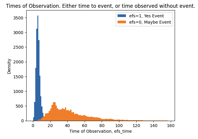

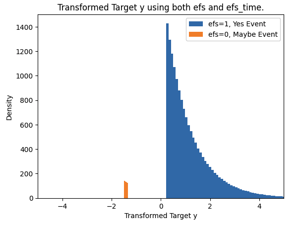
Transform Two Train Targets into One Target!

• Both targets efs and efs_time provide useful information.
• We will tranform these two targets into a single target to train our model with.
• In this competition we need to predict risk score.
• So we will create a target that mimics risk score to train our model.
• (Note this is only one out of many ways to transform two targets into one target. Considering experimenting on your own).

# 1. Set initial target value to efs_time
train["y"] = train.efs_time.values
# 2. Find maximum time of event cases (efs=1) and 
# minimum time of censored cases (efs=0)
mx = train.loc[train.efs==1,"efs_time"].max()
mn = train.loc[train.efs==0,"efs_time"].min()
# 3. Adjust time values for censored cases
# Add (mx - mn) to make all censored cases larger than event cases
train.loc[train.efs==0,"y"] = train.loc[train.efs==0,"y"] + mx - mn
# 4. Rank all values (starting from 1)
train.y = train.y.rank()
# 5. Make ranks of censored cases larger
# Add 2 times the data length to clearly differentiate
train.loc[train.efs==0,"y"] += 2*len(train)
# 6. Normalize to values between 0~1
train.y = train.y / train.y.max()
# 7. Apply log transformation
train.y = np.log(train.y)
# 8. Center mean to 0
train.y -= train.y.mean()
# 9. Reverse sign (to interpret as risk score)
train.y *= -1.0

plt.hist(train.loc[train.efs==1,"y"],bins=100,label="efs=1, Yes Event")
plt.hist(train.loc[train.efs==0,"y"],bins=100,label="efs=0, Maybe Event")
plt.xlim((-5,5))
plt.xlabel("Transformed Target y")
plt.ylabel("Density")
plt.title("Transformed Target y using both efs and efs_time.")
plt.legend()
plt.show()

 

 

Purpose of this transformation:

1. Clearly differentiate between censored cases and event cases
2. Transform values into appropriate range
3. Make it interpretable as risk scores (multiply by -1 at the end)

As a result:

• Event cases (efs=1) have higher risk scores
• Censored cases (efs=0) have lower risk scores
• Overall distribution becomes normalized

Detailed Explanation about #5 part:

# 5. Make ranks of censored cases larger
# Add 2 times the data length to clearly differentiate
train.loc[train.efs==0,"y"] += 2*len(train)

# Example data: 5 patients
# efs=1: Event occurred (death)
# efs=0: Censored (end of tracking)
# Initial data
Patient A: efs=1, efs_time=10  # Died on day 10
Patient B: efs=1, efs_time=20  # Died on day 20
Patient C: efs=0, efs_time=15  # Survival confirmed until day 15
Patient D: efs=1, efs_time=5   # Died on day 5
Patient E: efs=0, efs_time=25  # Survival confirmed until day 25
# After applying rank()
Patient D: 1  (shortest survival)
Patient A: 2
Patient C: 3
Patient B: 4
Patient E: 5  (longest survival)
# Adding 2*len(train) = 2*5 = 10 to censored cases
Patient D: 1      # efs=1, no change
Patient A: 2      # efs=1, no change
Patient C: 13     # efs=0, 3+10
Patient B: 4      # efs=1, no change
Patient E: 15     # efs=0, 5+10

Reasons for doing this:

1. Censored cases (efs=0) might have actually lived longer
2. Therefore, we make their ranks definitively larger
3. Adding twice the data length creates a large gap between efs=1 and efs=0 cases
4. This helps the model better distinguish between the two groups

Features

• There are a total of 57 features.
• From these 35 are categorical and 22 are numerical.
• Since most of the numerical features has only a few unique values, we will treat all features except donor_age and act_at_hct as categorical for our NN.
• So we will feed our NN 55 categorical features and 2 numerical features.

RMV = ["ID","efs","efs_time","y"]
FEATURES = [c for c in train.columns if not c in RMV]
print(f"There are {len(FEATURES)} FEATURES: {FEATURES}")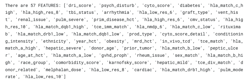

# Create empty list CATS - will store categorical variables
CATS = []
# Iterate through each feature (column) in FEATURES list
for c in FEATURES:
    # If the column's data type is "object" (strings etc.)
    if train[c].dtype=="object":
        # Fill missing values with "NAN" in both train and test
        train[c] = train[c].fillna("NAN")
        test[c] = test[c].fillna("NAN")
        # Add this column to CATS list
        CATS.append(c)
    
    # If it's a numerical column not containing "age" in its name    
    elif not "age" in c:
        # Convert numeric values to strings in both train and test
        train[c] = train[c].astype("str")
        test[c] = test[c].astype("str")
        # Add this column to CATS list
        CATS.append(c)
# Print the number and list of features treated as categorical
print(f"In these features, there are {len(CATS)} CATEGORICAL FEATURES: {CATS}")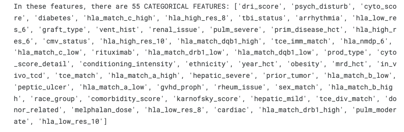

# Create lists to store categorical variable sizes and embedding dimensions
CAT_SIZE = []  # Number of unique values for each categorical variable
CAT_EMB = []   # Embedding dimensions for each categorical variable
NUMS = []      # List of numerical variables
# Combine train and test data
combined = pd.concat([train,test],axis=0,ignore_index=True)
print("We LABEL ENCODE the CATEGORICAL FEATURES: ")
# Iterate through all features
for c in FEATURES:
    # If it's a categorical variable
    if c in CATS:
        # Perform label encoding using factorize()
        combined[c],_ = combined[c].factorize()
        # Make minimum value 0
        combined[c] -= combined[c].min()
        # Convert to int32 type
        combined[c] = combined[c].astype("int32")
        
        # Calculate number of unique values and range
        n = combined[c].nunique()
        mn = combined[c].min()
        mx = combined[c].max()
        print(f'{c} has ({n}) unique values')
        
        # Store category size (max+1) and embedding dimension (sqrt(max+1))
        CAT_SIZE.append(mx+1)
        CAT_EMB.append( int(np.ceil( np.sqrt(mx+1))) )
    
    # If it's a numerical variable
    else:
        # Convert float64 to float32, int64 to int32 (memory optimization)
        if combined[c].dtype=="float64":
            combined[c] = combined[c].astype("float32")
        if combined[c].dtype=="int64":
            combined[c] = combined[c].astype("int32")
        
        # Perform standardization
        m = combined[c].mean()
        s = combined[c].std()
        combined[c] = (combined[c]-m)/s
        # Fill missing values with 0
        combined[c] = combined[c].fillna(0)
        
        # Add to numerical variables list
        NUMS.append(c)
# Split back into train and test
train = combined.iloc[:len(train)].copy()
test = combined.iloc[len(train):].reset_index(drop=True).copy()

We LABEL ENCODE the CATEGORICAL FEATURES: 
dri_score has (12) unique values
psych_disturb has (4) unique values
cyto_score has (8) unique values
diabetes has (4) unique values
hla_match_c_high has (4) unique values
hla_high_res_8 has (8) unique values
tbi_status has (8) unique values
arrhythmia has (4) unique values
hla_low_res_6 has (6) unique values
graft_type has (2) unique values
vent_hist has (3) unique values
renal_issue has (4) unique values
pulm_severe has (4) unique values
prim_disease_hct has (18) unique values
hla_high_res_6 has (7) unique values
cmv_status has (5) unique values
hla_high_res_10 has (9) unique values
hla_match_dqb1_high has (4) unique values
tce_imm_match has (9) unique values
hla_nmdp_6 has (6) unique values
hla_match_c_low has (4) unique values
rituximab has (3) unique values
hla_match_drb1_low has (3) unique values
hla_match_dqb1_low has (4) unique values
prod_type has (2) unique values
cyto_score_detail has (6) unique values
conditioning_intensity has (7) unique values
ethnicity has (4) unique values
year_hct has (13) unique values
obesity has (4) unique values
mrd_hct has (3) unique values
in_vivo_tcd has (3) unique values
tce_match has (5) unique values
hla_match_a_high has (4) unique values
hepatic_severe has (4) unique values
prior_tumor has (4) unique values
hla_match_b_low has (4) unique values
peptic_ulcer has (4) unique values
hla_match_a_low has (4) unique values
gvhd_proph has (18) unique values
rheum_issue has (4) unique values
sex_match has (5) unique values
hla_match_b_high has (4) unique values
race_group has (6) unique values
comorbidity_score has (12) unique values
karnofsky_score has (8) unique values
hepatic_mild has (4) unique values
tce_div_match has (5) unique values
donor_related has (4) unique values
melphalan_dose has (3) unique values
hla_low_res_8 has (8) unique values
cardiac has (4) unique values
hla_match_drb1_high has (4) unique values
pulm_moderate has (4) unique values
hla_low_res_10 has (8) unique values

TensorFlow NN

• We train NN model with CV 0.670

import tensorflow as tf
from tensorflow.keras.models import Model
from tensorflow.keras.layers import Dense, Dropout, Input, Embedding
from tensorflow.keras.layers import Concatenate, BatchNormalization
import tensorflow.keras.backend as K
from sklearn.model_selection import KFold

print('TF Version',tf.__version__)

Learning Schedule

# Set total 4 epochs
EPOCHS = 4
# Define learning rate for each epoch
LRS = [0.01]*2 + [0.001]*1 + [0.0001]*1
# Written out: LRS = [0.01, 0.01, 0.001, 0.0001]
# Function that returns learning rate for each epoch
def lrfn(epoch):
    return LRS[epoch]
# Create list of epoch numbers (0 to 3)
rng = [i for i in range(EPOCHS)]
# Create list of learning rate values for each epoch
lr_y = [lrfn(x) for x in rng]

plt.figure(figsize=(10, 4))
plt.plot(rng, lr_y, '-o')
print("Learning rate schedule: {:.3g} to {:.3g} to {:.3g}". \
        format(lr_y[0], max(lr_y), lr_y[-1]))
plt.xlabel("Epoch")
plt.ylabel("Learning Rate")
plt.title("Learning Rate Schedule")
plt.show()

lr_callback = tf.keras.callbacks.LearningRateScheduler(lrfn, verbose = False)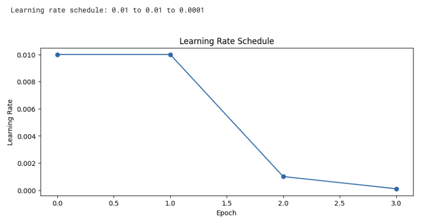

• Learning Rate Schedule:
  
  • First 2 epochs: 0.01 (fast learning with high learning rate)
  • 3rd epoch: 0.001 (decreased learning rate)
  • 4th epoch: 0.0001 (fine-tuning with smaller learning rate)
• Reasons for gradually decreasing the learning rate:
  1. Fast learning with large learning rate initially
  2. Fine-tuning with small learning rate in later stages
  3. This helps the model converge more stably

Model Definition

• We use embedding layers for all label encoded categorical features.
• Then we concatenate all categorical embeddings with the numerical features.
• We create an MLP with two hidden layers.
• Our final output layer has one linear neuron and during training we use MSE loss with Adam optimizer.

def build_model():
    # 1. Handle categorical variables
    # Create input layer for categorical variables
    x_input_cats = Input(shape=(len(CATS),))
    embs = []
    
    # Create embedding layer for each categorical variable
    for j in range(len(CATS)):
        # Create embedding layer (input size: CAT_SIZE[j], output size: CAT_EMB[j])
        e = tf.keras.layers.Embedding(CAT_SIZE[j], CAT_EMB[j])
        # Apply embedding to j-th categorical variable
        x = e(x_input_cats[:,j])
        # Flatten embedding result to 1D
        x = tf.keras.layers.Flatten()(x)
        # Store embedding result
        embs.append(x)
    
    # 2. Handle numerical variables
    # Create input layer for numerical variables
    x_input_nums = Input(shape=(len(NUMS),))
    
    # 3. Combine categorical and numerical features
    # Connect all embedding results and numerical variables
    x = tf.keras.layers.Concatenate(axis=-1)(embs+[x_input_nums])
    
    # 4. Add fully connected layers (Dense)
    # Hidden layer with 256 neurons (ReLU activation)
    x = Dense(256, activation='relu')(x)
    x = Dense(256, activation='relu')(x)
    # Output layer with 1 neuron (linear activation)
    x = Dense(1, activation='linear')(x)
    
    # 5. Create model
    # Input: categorical and numerical variables
    # Output: predicted value
    model = Model(inputs=[x_input_cats,x_input_nums], outputs=x)
    
    return model

• linear activation: f(x) = x
  • Outputs input value as is
  • No transformation applied
  • Characteristics:
    • Unlimited output range (-∞ ~ +∞)
    • Commonly used in output layer for regression
    • Suitable for continuous real value prediction
• ReLU (Rectified Linear Unit) Activation: f(x) = max(0, x)
  • Outputs 0 for negative values, keeps positive values as is
  • Characteristics:
    
    • Output range: [0, ∞)
    • Most commonly used in hidden layers
    • Reduces vanishing gradient problem
    • Simple and fast computation
• Linear:        ReLU:
      ↗           ↗
    ↗           _/
  ↗           _/

Train K Fold

• We train our NN below.
• If you want to save the trained model weights, you can uncomment the commented lines below.

%%time

REPEATS = 3
FOLDS = 5
kf = KFold(n_splits=FOLDS, random_state=42, shuffle=True)

oof_nn = np.zeros( len(train) )
pred_nn = np.zeros( len(test) )

#directory = "checkpoints"
#if not os.path.exists(directory):
#    os.makedirs(directory)

for r in range(REPEATS):
    VERBOSE = r==0
    print("#"*25)
    print(f"### REPEAT {r+1} ###")
    print("#"*25)
        
    for i, (train_index, test_index) in enumerate(kf.split(train)):
        
        X_train_cats = train.loc[train_index,CATS].values
        X_train_nums = train.loc[train_index,NUMS].values
        y_train = train.loc[train_index,"y"].values
        y_train2 = train.loc[train_index,"efs"].values
        
        X_valid_cats = train.loc[test_index,CATS].values
        X_valid_nums = train.loc[test_index,NUMS].values
        y_valid = train.loc[test_index,"y"].values
        y_valid2 = train.loc[test_index,"efs"].values
        
        X_test_cats = test[CATS].values
        X_test_nums = test[NUMS].values

        if VERBOSE:
            print(" ","#"*25)
            print(" ",f"### Fold {i+1} ###")
            print(" ","#"*25)
        
        # TRAIN MODEL
        K.clear_session()
        model = build_model()
        model.compile(optimizer=tf.keras.optimizers.Adam(0.001), 
                      loss="mean_squared_error",  
                     )
        v = 2 if VERBOSE else 0
        model.fit([X_train_cats,X_train_nums], [y_train], 
                  validation_data = ([X_valid_cats,X_valid_nums], [y_valid]),
                  callbacks = [lr_callback],
                  batch_size=512, epochs=EPOCHS, verbose=v)
        #model.save_weights(f'{directory}/NN_f{i}_r{r}.weights.h5')
        
        # INFER OOF
        oof_nn[test_index] += model.predict([X_valid_cats,X_valid_nums], verbose=v, batch_size=512).flatten()
        # INFER TEST
        pred_nn += model.predict([X_test_cats,X_test_nums], verbose=v, batch_size=512).flatten()

oof_nn /= REPEATS
pred_nn /= (FOLDS*REPEATS)

Compute Overall Metric

from metric import score

y_true = train[["ID","efs","efs_time","race_group"]].copy()
y_pred = train[["ID"]].copy()
y_pred["prediction"] = oof_nn
m = score(y_true.copy(), y_pred.copy(), "ID")
print(f"\nOverall CV for NN =",m)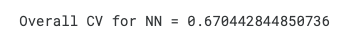

Create Submission CSV

sub = pd.read_csv("/kaggle/input/equity-post-HCT-survival-predictions/sample_submission.csv")
sub.prediction = pred_nn
sub.to_csv("submission.csv",index=False)
print("Sub shape:",sub.shape)
sub.head()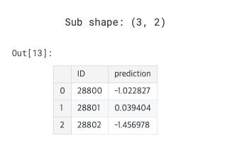

---

게으른 천재는 그냥 게으름뱅이일 뿐이다.